Power and precision

Why the push for replacing “power” with “precision” is misguided

[Code for all the plots in this post is available in this gist.]

One of the common claims of anti-significance-testing reformers is that power analysis is flawed, and that we should be planning for study “precision” instead. I think this is wrong for several reasons that I will outline here. In summary:

• “Precision” is not itself a primitive theoretical concept. It is an intuition that is manifest through other more basic concepts, and it is those more basic concepts that we must understand.
• Precision can be thought of as the ability to avoid confusion between closeby regions of the parameter space. When we define power properly, we see that power is directly connected to precision. We don’t replace power with precision; we explain precision using power.
• Expected CI width (which some associate with “precision”) can depend on the parameter value, except in special cases. Power analysis directs your attention to a specific area of interest, linked to the purpose of the study, and hence overcomes this problem with CI-only concepts of precision.
• (One-tailed) Power is a flexible way of thinking about precision; confidence intervals (CIs), computed with equal probability in each tail, have difficulties with error trade-offs (asymmetricly-tailed CIs, though possible, would surely confuse people). We should thus keep the concept of power, and explain CIs and precision using confusion/error as the primitives.

Power is misunderstood

For reasons I don’t quite understand, power is one of the most-confused concepts among users of statistics. The reasons are probably some combination of the difficulty of probabilistic thinking, cookbook stats teaching, and the pressures involved in research that make statistics into performance art rather than a research tool.

What is often called “power analysis” is not closely related, conceptually, to power analysis in frequentist statistics. Looking at a past study’s observed effect size, assuming that is the true effect size and plugging it into a piece of software, and computing the sample size that will yield 20% chance of missing that effect? That’s not really a power analysis in any useful sense.

So, definitely: power analysis is misunderstood, and planning for precision, as suggested by pro-interval reformers (e.g. Rothman and Greenland, 2018) is superior to the performative “power analyses” that are often done. What I will argue here is that what is even better is to use the real, frequentist concept of power.

This may not actually be a point of disagreement with some interval advocates, e.g. Greenland, at least. In his recent paper on significance tests (Greenland, 2019), he advocates the use of valid p values (in the guise of surprisal values, log₂(p)), and that “confidence intervals have not provided the hoped-for cure for testing abuse, but have instead perpetuated the dichotomania and excessive certainty that plague research reports.”

“Precision” is not a primitive theoretical concept

What is precision? In statistics, there is a one formal definition of precision: the reciprocal of the variance of a distribution. But this isn’t really what people mean when they say “precision,” which is a typically evaluation of the “information” in the data, or the expected informativeness of data from a particular design.¹

How many ways can we think about study planning for precision?

1. Expected confidence interval width; but what confidence level, and why? And for which assumed true parameter value?
2. Standard deviation of the sampling distribution of an estimator (standard error). This need not be related to the CI width; see Morey et al (2016).
3. Fisher information (the curvature of the log-likelihood function), but for what true parameter?
4. Expected posterior standard deviation (Bayesian), but do we want dependence on the prior for planning?
5. Expected posterior credible interval/highest posterior density; but again what credible level, and why? (Bayesian)
6. Expected size of a Bayes factor (Bayesian)

There are others. Given that this blog post is not about Bayesian methods, I’ll just point people elsewhere (1, 2, 3; but note that the descriptions of classical power in these references are not generally correct).

Given that there are multiple ways we can think about “precision” even in the classical/frequentist paradigm, we have to choose one. Confidence intervals have been suggested, but what confidence level? And do we use an expected width for a single parameter, average over a range of parameters (pseudo-Bayesian), or a “worst case” width? Why?

I will consider an intuitive definition of “precision” and show that power does, in fact, connect directly with that definition. Moreover, confidence intervals are directly connected with that definition. This grounds precision in “error”, a frequentist primitive notion, as well as telling us why and how we should use CIs for precision.

A definition of “precision”

Precision is the tendancy for confusions between close parts of the parameter space to be rare. Higher precision means that closer and closer parts of the parameter space can be distinguished.

For instance, an imprecise radar gun may rarely confuse people driving below the speed limit (30mph) with those speeding at over 50mph, but may often confuse someone driving the speed limit with someone speeding at over 40mph. A more precise radar gun may rarely confuse non-speeders with those going over 35mph. A radar gun is called imprecise when it tends to confuse slower speeds with faster speeds (and vice versa).

Precision — from a design perspective, at least — is concerned with confusions or errors, and one’s tendency to commit them for nearby parameter values.

A brief power primer

Suppose you are trying to tell whether a parameter — call it θ — is “large”. For our purposes, we don’t need to define “large” now. We assume we can find a statistic, X, that carries the evidence regarding θ. How we know that X carries the evidence about θ is a technical issue, but for most problems is uncontroversial and we are familiar with many evidence/parameter pairs (Z,p; δ,t; ∑δᵢ²,F; etc). The key feature of these statistics is that for a given design/sample size, as the statistic gets larger, there is greater and greater evidence that the parameter is not small. As |t| gets larger, we have greater evidence against the hypothesis that the difference between two means is small (and vice versa: when |t| is smaller, we have greater and greater evidence against the hypothesis that δ is large). This does not depend on any particular definition of “large” or “small”.

(Everything here will be explained with one-sided tests. You may be used to thinking about two-sided tests, but it is better to ground your thinking in one-sided tests because they are conceptually simpler. Two-sided tests and confidence intervals can be formed from two one-sided tests in opposite directions.)

Back to our hypothetical statistic, X: Suppose that whenever X is bigger than some number, X≥c, I’ll say “This is strong enough evidence to say that θ is large [at least tentatively].” I think we can all agree that this would be reasonable for some c and some definition of “large” θ. We have to interpret the statistical evidence somehow. We can finesse things a bit and say that this is evidence that “θ is not small” (there might be other evidence lurking that our statistical model is flawed, so θ might be a something we abandon altogether), but the idea is the same, for our purposes.

For a given design, a power curve is just the probability that X≥c, for all possible θ values. To make things concrete, suppose that we’ve got 100 binomial trials, and our criterion is X≥60 — so, when X is at least 60, we’re going to say that our binomial probability is “large”. Figure 1 shows the corresponding power curve, Pr(X≥60; p).

Figure 1: The power curve for X≥60 in a binomial setting with N=100.

We can immediately read several things from the power curve in Figure 1.

1. First, we can see that we would almost never see an observation as large as 60 when p<0.5 or so.
2. X≥60 serves as an α=.05 test of the hypothesis p≤.51, because if p≤.51, we would rarely (with probability less than .05) see an observation as large.
3. If we wanted an α=.01 level test, this criterion would serve for the hypothesis p≤.48.
4. Generally, we can assess what the good inferences would be for any error tolerance.

We can also read the consequences of not meeting the criterion. Failing to meet the criterion — X<60 — would lead us to infer that p<.7 or so (depending on how tolerant of error we are). If p≥.7, we would almost surely see X≥60; so if we didn’t see X≥60, we’d say p<.7 (ish). This is all straightforward significance testing logic, but crucially, it is something people forget about power analysis. Yes, power analysis can help you pick a sample size; but power is also intimately tied to how you interpret results.

This makes plain the problem with the common argument that significance tests say nothing about the effect size: it simply isn’t true (or, somewhat more accurately: it is only true if you don’t use significance tests well).

Figure 2: The power curve for X≤60 in a binomial setting with N=100.

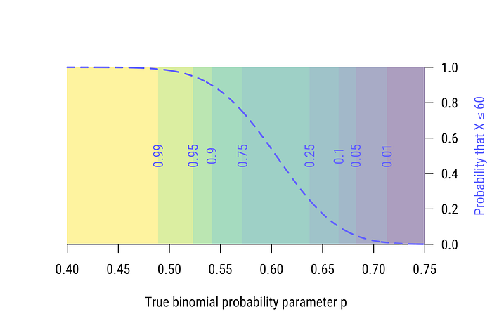
Figure 2 shows a second power curve: one corresponding to the criterion X≤60. We can read directly off the power curve that X≤60 would serve as a good criterion for a test of the hypothesis p≥.7 or so. If p≥.7, we’d almost never see X≤60; so when see X≤60, we infer that p<.7. On the other hand, when we fail to see X≤60 — that is, X>60 — we infer that p>.5 or so (again, depending on our tolerance for error).

Fact 1: Power curves tell us what we can infer when we either see, or don’t see, observations that meet some criterion.

Figure 3: Figures 1 and 2 combined, along with (horizontal lines, top to bottom: 50%, 80%, 90%, and 98% CIs, when X=60)

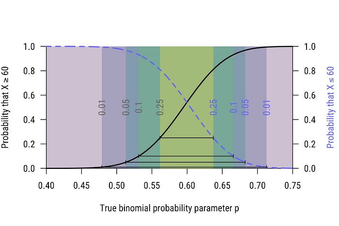
If you’re primed to think in terms of confidence intervals, you can probably see where this is going. Figure 1 tells us what happens when our criterion is X≥60; Figure 2 tells us what happens when X≤60. So what happens when X=60, which is where both criterion are met? We use the black line to give us a lower bound on our inference, and the blue line to give us an upper bound. We can read every confidence interval directly off the power curves. I’ve selected the 50%, 80%, 90%, and 98% confidence levels, and plotted the them on Figure 3 (you can verify this for yourself with, say, binom.test(x=60, n=100, conf.level = .5) in R and looking at the resulting 50% CI).

Fact 2: Power curves are directly related to confidence intervals. You can determine what the CI would be for any observation by setting up power curves with that observation as a criterion. (This also directly relates power curves and CIs to p values. Properly understood, all three are just different perspectives on general significance testing logic.)

So what is the purpose of a power analysis in the design stage of a study? A power analysis we decide where in the parameter space to focus by setting up a “null” hypothesis (e.g., p≤1/3, or μ≥0). We then choose our sample size and a criterion such that when our criterion is met, we will be able to infer that the parameter is not in the location where the power curve is low, and when the criterion is not met, the parameter is not in the region where the power curve is high.

You can probably already see: powering a study is explicitly deciding on a “precision”, focused on an important area of the parameter space. The “precision” is given by the distance between the very low and very high parts of the power curve, where “very” is determined by our tolerance for error (or, if you prefer, confidence level). The statistical primitive is “error,” the foundation of the significance test and the confidence interval.

Figure 4: The parameter space divided into regions, “small” and “large”. A significance test with these regions, and the criterion X≥60, will rarely confuse a “small” parameter for a “large” one. It will almost always label a “reliably-detectably-large” parameter as “large”. Confusions are common for parameter values between “small” and “reliably-detectably-large”.

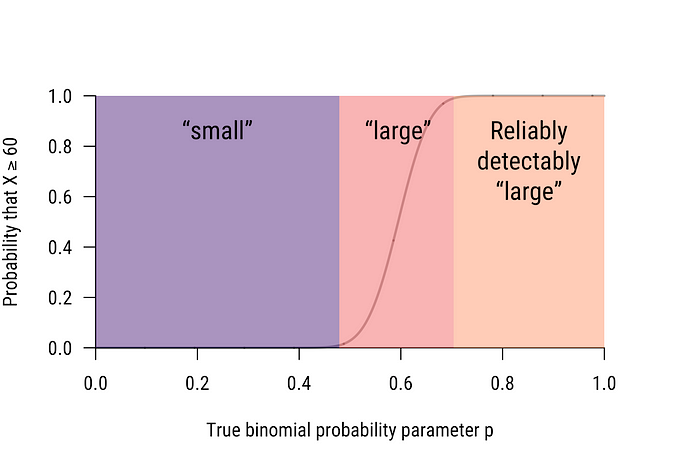
To make this clearer, look at Figure 4, which shows the entire parameter space divided into “small” (which would often be called “null”) and “large”, with “large” futher subdivided into “large” and “reliably-detectably large”. Confusions (“errors”) are only likely for values outside of the “small” and “reliably-detectably large” parameter ranges. As we will see in the next section, increasing the sample size increases the slope of the power function, hence decreasing the width of this confusion-prone region. This corresponds directly to increased precision.

Planning a study using power

To make things simple for now, we consider a one-sample t test. The one-sample normal case has many nice features, including familiarity, continuous data,² and a roughly constant standard error across the parameter space (the standard error of the standardized effect size is about 1/√n). We’ll start with this example, then break the intuitions with a less well-behaved example later.

Suppose we’re interested in telling positive from negative effect sizes, so we set up a standard one-sided test (α=0.025) that rejects when t≥2 (give or take, depending on n). We’re interested in planning our study, so we want to pick a sample size.

Figure 5: The power curve for a one-sample t-test for the criterion t≥2, when n=100, as a function of the standardized effect size δ.

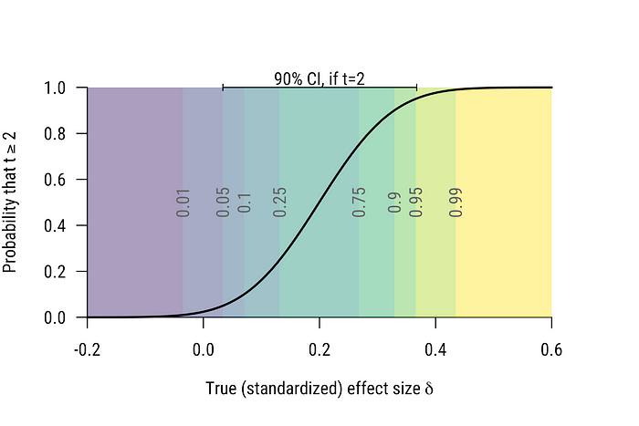
The power curve for n=100 is shown in Figure 4. Again, we can read confidence intervals directly off the power curve. If t=2 (exactly the criterion) the 90% confidence interval will extend from the parameter to which there is 5% power up to the parameter to which there is 95% power.

We can also consider α=0.025. When t=2, the result is just on the edge of “significance” and “nonsignificance” at α=0.025 so the power curve tells us what we can infer in case of significance (δ is at least 0) and nonsignificance (δ is at most 0.4). The 95% confidence interval when t=2 will therefore run from 0 to 0.4.

When planning, people typically make one or more of several mistakes:

1. They forego a design analysis altogether, and pick their sample size based on what others typically use
2. They pick an observed effect size from the literature, and compute power assuming this effect size (note that among other things, this is a confusion of statistic and parameter, and will generally lead to imprecise designs)
3. They use 80% power without thinking about why

I’ll argue later that the ability to choose your power probability is actually a good thing and makes power analysis more flexible than CIs (where the tail probabilities are equal). But for now: why 80%? This is supposed to reflect a tradeoff between error rates (so-called “Type I” errors typically considered worse than “Type II”) but usually, people are interested in simply drawing an inference about the parameter. There are no definite costs for the associated “errors”; these errors are devices we use for thinking about the problem of inference.

There’s usually no good reason for our two inferences (“the effect size is bigger than θₗ” and “the effect size is smaller than θᵤ”) to be governed by different “error” rates because the error tolerance is simply a device to formalize a general conservatism toward the inference.

Figure 5 shows the problem with using 80% without thinking about why: we almost never tolerate a 20% error rate for inference. When we draw our inference we’ll adopt a more conservative upper bound (probably based on an α=0.025 test, or equivalently, a 95% CI, but it doesn’t really matter for the point), and so a “nonsignificant” result may not allow us to rule that the effect size is as large as we “powered” to. A “power analysis” based on tolerating a 20% upper-bound error rate yields designs that are irrelevant to our eventual inference; the range of effect sizes we can rule out on the top end will be smaller than what we would like. It’s usually just bad planning.

Unless we have some reason to specify error trade-offs, we’ll look at two points on the power curve especially: the one that yield α power, and the one that yields 1-α power. Where power is α defines the division between “small” and “large” (or, if you like, “null” and “alternative”). Above the effect sizes with 1-α power are the “reliably-detectably large” effect sizes. Between the two is the confusable range.

Figure 6: Relationship between the power curve as N increases and the confidence interval when is exactly equal to the significance criterion. The criterion is adapted as sample size increases to yield an α=0.025 test for δ<0. Horizontal dashed lines are at powers α=0.025 and 1-α=0.975.

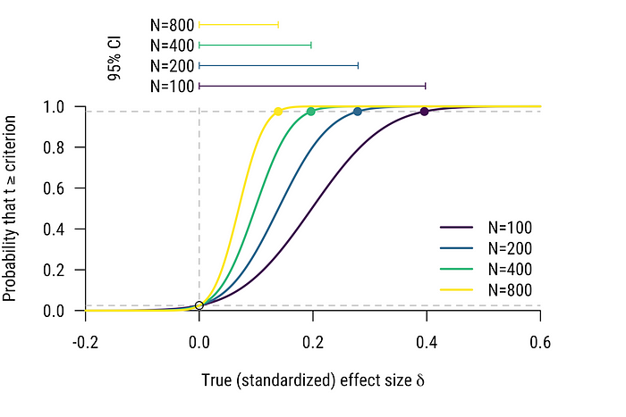
Fact 3: The width of the 100(1–2α)% confidence interval when the evidence is at the significance criterion is exactly the width of the confusable region in the α one-sided test (but see footnote 2 for a slight caveat with discrete data).

Figure 6 shows Fact 3 clearly and how it is affected by an increase in sample size. Most people are aware that when the test is just significant, the CI will just touch the “null” value. With the additional knowledge that the other bound just touches the reliably-detectably-different range where power is above 1-α, you can read the CI directly off the power curve.

This is all just based on significance testing logic; the significance test and CI are based on the same logic, and hence show this elegant symmetry.

It is now clear how to plan for precision using power. Choose an effect size you’d like to reliably (with probability 1-α) say is “large” (if you like, “non-null”) with a one-sided test. The difference between this value and your “null” value is the precision. This precision is also the width of the CI when the data are just significant. Find a sample size such that your power curve is suitably high (1-α) for effect sizes you’d like to be reliably detectable.

You can do this analysis with any power analysis software. A desire for precision doesn’t mean you should abandon power analysis: just the opposite, in fact. A desire for precision tells you why power analyses are useful, and a proper understanding of power shows how power and CIs are intimately connected.

Why not just use confidence intervals?

Proponents of confidence intervals may take the above as evidence that we can just get away with using the confidence interval definition of precision. Didn’t I show that the confidence interval width is the precision?

Yes, but the crucial question is which confidence interval width. The confidence interval width I gave above is specifically the one constructed using the confusible region of the parameter space, as determined by a test. For some tests, this doesn’t much matter, because the expected confidence interval length is roughly the same throughout the parameter space. In fact, for the normal distribution, the mean and standard error are completely uncorrelated. Because CI advocates almost always use examples with normal distributions, we are often fooled into thinking that this is generally true.

It isn’t.

When we move beyond the easy normal world, into binomials, poisson, negative binomials, gammas, betas, etc, things get more complicated. The expected width of a CI is related, sometimes strongly, to the parameter value of interest.

Consider an example. Suppose we are conducting a poll to determine support for a political issue. We decide on an open-ended design, where we will randomly call people until we reach a certain number of people who agree (“yes”, or a “success”). This threshold number of successes is called the “size” of our design. We will use the total number of failures (“no”) we encounter before reaching our threshold size to estimate the probability of a success (the proportion of “yes” votes in the population, parameter p). These outcomes are modeled by a negative binomial distribution.

Notice that the more failures we encounter, the smaller we believe the true probability of a success is.

Figure 7: Confidence intervals for outcomes from 0 to 50 from two negative binomial designs: size=1 (top) and size=25 (bottom). Parameter p is the probability of a success.

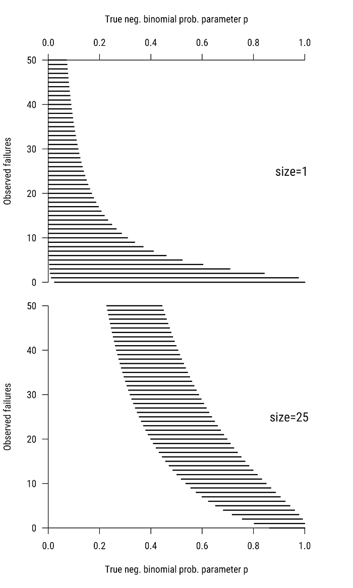
Figure 7 shows the two-sided 95% confidence intervals corresponding to every potential outcome from 0 to 50 for two designs: sizes of 1 (top) and 25 (bottom). Notice that the design with size 25 is equivalent to running the size 1 design 25 times in a row and adding up the total failures. So increasing the negative binomial size is analogous to increasing sample size in fixed n designs.

Figure 7 clearly shows that when it takes only a few failures to reach our criterion, we infer that there are more “yes” voters in the population (true p is large). When we see more failures on the way to our criterion, we infer a smaller p. But the CIs are not equal width; they are not even close. When the size is 1 (top) and our first call is a “yes” (we meet our criterion without any failures) we get very little information about p, except that it obviously can’t be very small. When the number of failures is larger, our CI is shorter as our inference “bunches up” near p=0.

On the other hand, when the size is 25 (bottom), if we observe no failures on our way to out criterion of 25 “yes” votes, we infer that the probability of “yes” must be very high. The width of our CI increases as the number of failures increases, and eventually decreases again. Crucially, how wide we expect the CI to be depends on what we believe p is, but p is precisely the thing we don’t know and want to find out.

Why don’t we just make a guess at p? This would give us an expected CI width for any size we like (for instance, when size is 25 and p=0.6, the 95% CIs will be width about 0.30, on average; for p=0.2, the average width is 0.14). We could do this, but what if we were wrong? A better approach is to think about what the purpose of our study is, and what we’d like to infer. Is it important to be able to test whether p<.5 (that is, the majority supports “no”)? What is the most important part of the parameter space? For what values should we have sufficient precision?

What we can do is to set up a test in that interesting region. Note that where we think the parameter is, and where the interesting region is, are not the same; to think they are the same is another fallacy of power. We might well think that the probability of a success is very low, and hence we’ll get a lot of information even with size of 1 (our CI will be narrow; Figure 7, top panel). But if we’re wrong and the probability of success is relatively high, we are in danger of getting almost no information (particularly if our first observation is “yes”). We need a power analysis, guided by what we’d like to infer or learn.

Figure 8: Power curves for sizes 1, 10, 25, and 50 for the negative binomial example, and corresponding 95% CIs when the observation is just on the significance criterion. Slight variations in the upper bounds of the CIs are due to discreteness of the data (see also Footnote 3).

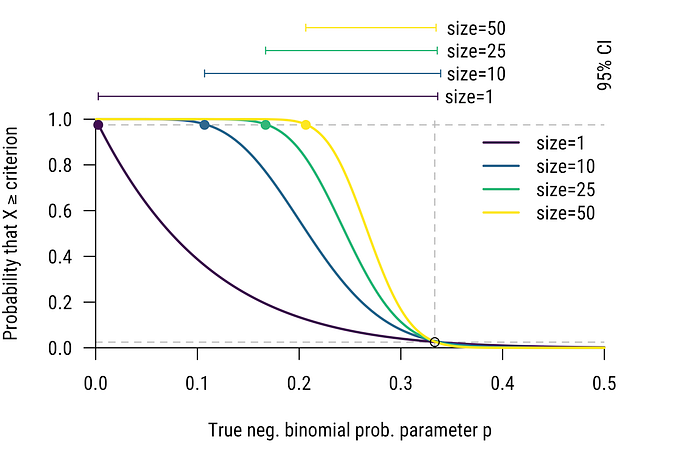
Suppose that our survey was about public support for a political candidate who is considering dropping out of race if their support is too low in the polls; by default they will stay in the race. We operationalize “too low” support as below 1/3. (that is, the true p<1/3). Figure 8 shows the power curves for the α=0.025 test for sizes 1, 10, 25, and 50, and the corresponding 95% CIs.³

Both the power curve and the CIs, of course, tell the same story: these designs are terrible, and the confusability region is large even for a size of 50. The precision of the design is likely not very good for the purpose at hand (at least, if one accepts the α=0.025. Choice of α is always arguable, and particularly in this practical example. It is easy, however, to adjust one’s tolerance for error and when plotting power curves.)

Planning with power is more flexible than (typical) CI use

Above, I’ve shown that CIs and power curves are intimately related, and that properly planning a design using power curves is, in fact, planning with confidence intervals. As I alluded to previously, however, there are cases where it is difficult to use CIs — at least, the way they’re typically computed — and easier to use power curves.

Studies can be designed with asymmetric tests in mind: in fact, this is often how we present power, although we almost never use this fact in practice (e.g., we still use an α=0.025 upper bound on the CI even though we designed our study using a 20% error tolerance on the upper bound). If we power 80% to effect size θ₁, what this implies is that when I get a non-significant effect, I’m happy to infer that θ<θ₁ (even with the 20% error attached to this inference). Maybe in the candidate resigning example above, asymmetric would be appropriate: dropping out of a race is permanent, so one should be careful to be conservative (in the error sense) in assessing the upper bound on support; inferring that support is higher than it is, the worst that can happen is more stressful days running and then losing the inevitable vote to one’s opponent.

Although I can’t think of many such examples in basic science, the nice thing about power reasoning is that this is easily allowed, and may be crucial to planning in some cases. What of confidence intervals? The typical α=0.025, β=.2 setup is equivalent to a CI built out of two one-tailed CIs: one having error rate 0.025, and the other 0.2. This leads to an asymmetricly-tailed, 77.5% CI. When θ=θ₁, there will be a 20% chance that the upper CI bound dips below θ₁. Due to the symmetry between CIs and tests, this is will work, but it is inconsistent with how CIs are used and interpreted. The CI interpretation doesn’t seem to add anything to the planning process.

Conclusion

You can perform the above analyses with any program that computes power (look at the one-sided 1-α point on the power curve for a given sample size) or confidence intervals (compute the width of the CI given an observation that would be just significant for a given sample size and confidence coefficient).

Properly planning a study using power is, in fact, planning for precision. When precision is defined intuitively in terms of confusions or errors (i.e. not simply associated with CIs by definition) we see that precision arises from power reasoning quite easily. Moreover, the connection to CIs is made explicit, instead of assumed.

[Code for all the plots in this post is available in this gist.]

Footnotes

¹ The precision of a posterior distribution can be used by a Bayesian as a post-data measure of precision, but it isn’t the only way a Bayesian can think about the information in the data.☝

² With continuous data, the left- and right- tailed power curves are mirror images of one another, so we only need one of them. The discrete data in the first binomial example meant that we needed two power curves — a right-tailed and a left-tailed test, the black and blue curves — to get the exact confidence intervals. For discrete data, they are usually almost mirror images, but not quite.☝

³ These CIs were computed properly using two one-sided tests, but unlike with the continuous data example, the points on the power curves at 1-α will not exactly correspond to the endpoints of the CI due to the discreteness of the data (one is computed with X<c, the other with X≤c). To simplify exposition, I did not add the opposing one-tailed power curve as I did in the first example. But the closeness of agreement between the endpoints of the CI and the points on the power curve should suffice to show that the differences due to discreteness are very small.☝